RayTracer

My cornell box (2K resolution image with 300 samples per pixel)

During my master’s year I learnt about different rendering paradigms. I was smitten by ray tracing’s simple concept and the rendering equation, so building a ray tracer and implementing some of the many techniques I read about has been a goal of mine ever since. This application stems from a piece of coursework for my 4th year rendering module which, although enough for an honorable mark, was inaccurate, clunky, and slow. This project has been and still is a great way for me to deepen my knowledge of computer graphics, 3D maths and C++ programming.

My first task was to refactor the 3D maths used in the application, the data structures and routines, to be faster and more accurate. These include vectors, quaternions and matrices. I started with common optimisations such as loop-unravelling, using bitwise operations or unsigned integer arithmetic to minimise CPU cycles. Agner Fog’s C++ optimisation guides are a treasure trove of information for explaining these tricks.

I also researched SIMD parallelism and vectoried some of my maths data structures using the built-in intrinsics in xmmintrin.h. This reduces the number of operations needed resulting in better CPU usage and a drastic speed-up (in my case a 200% speed-up for tasks such as matrix multiplication or vector addition).

// transpose a 4x4 matrix
Matrix4 Matrix4::transpose(const Matrix4& mat) 
{
    __m128 c0c1 = _mm_shuffle_ps(mat.__m[0], 
        mat.__m[1], _MM_SHUFFLE(1, 0, 1, 0));
    __m128 c2c3 = _mm_shuffle_ps(mat.__m[2], 
        mat.__m[3], _MM_SHUFFLE(1, 0, 1, 0));
    __m128 c1c0 = _mm_shuffle_ps(mat.__m[1], 
        mat.__m[0], _MM_SHUFFLE(2, 3, 2, 3));
    __m128 c3c2 = _mm_shuffle_ps(mat.__m[3], 
        mat.__m[2], _MM_SHUFFLE(2, 3, 2, 3));
    Matrix4 t;
    t.__m[0] = _mm_shuffle_ps(c0c1, c2c3, 
        _MM_SHUFFLE(2, 0, 2, 0));
    t.__m[1] = _mm_shuffle_ps(c0c1, c2c3, 
        _MM_SHUFFLE(3, 1, 3, 1));
    t.__m[2] = _mm_shuffle_ps(c1c0, c3c2, 
        _MM_SHUFFLE(1, 3, 1, 3));
    t.__m[3] = _mm_shuffle_ps(c1c0, c3c2, 
        _MM_SHUFFLE(0, 2, 0, 2));
    return t;
}

C++ code for matrix transpose with intrinsics.

I am now the proud owner of a small 3D maths library called Thomath that I use in my graphics projects!

I also wrote my own WaveFrontOBJ file parser, using the .obj files exported by Blender as templates so that I may easily create my own custom 3D models and render them. The current verion uses modern C++ features such as regular expressions to split file lines into STL vectors and strings, but because of it’s heavy use of heap allocation I think I will revert to a more C based solution in the future.

Clockwise: correct UVs, random directions, normals. Generated in the old application.

As my application grew in size and complexity, I quickly found myself hindered by the limitations of my development environment. My original coursework used OpenGL 1.1 (which can be carbon dated to the Jurassic era) and, due to its much smaller scope, was manageable on my small Linux partition with no IDE and no external libary dependencies bar the Qt GUI library.

Once I could raytrace objects, I migrated the project to a Windows environment to use Visual Studio and modern OpenGL 4.5 features.
To manage the third party libraries I would now need, I learnt to use CMake to manage my project and wrote a script to generate Visual Studio solutions. Adding external code is now much easier and requires only editing a CMakeList file and running the script, no arcane Visual Studio knowledge needed!

I used this change as an occasion to make deep modifications to the application’s architecture, such as using Dear ImGui instead of Qt for the GUI, so much so that practically nothing of the original coursework remains.

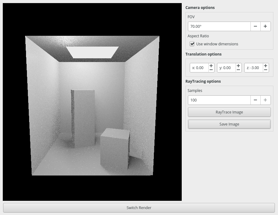
Top to bottom: Original GUI in Linux, new GUI in Windows.

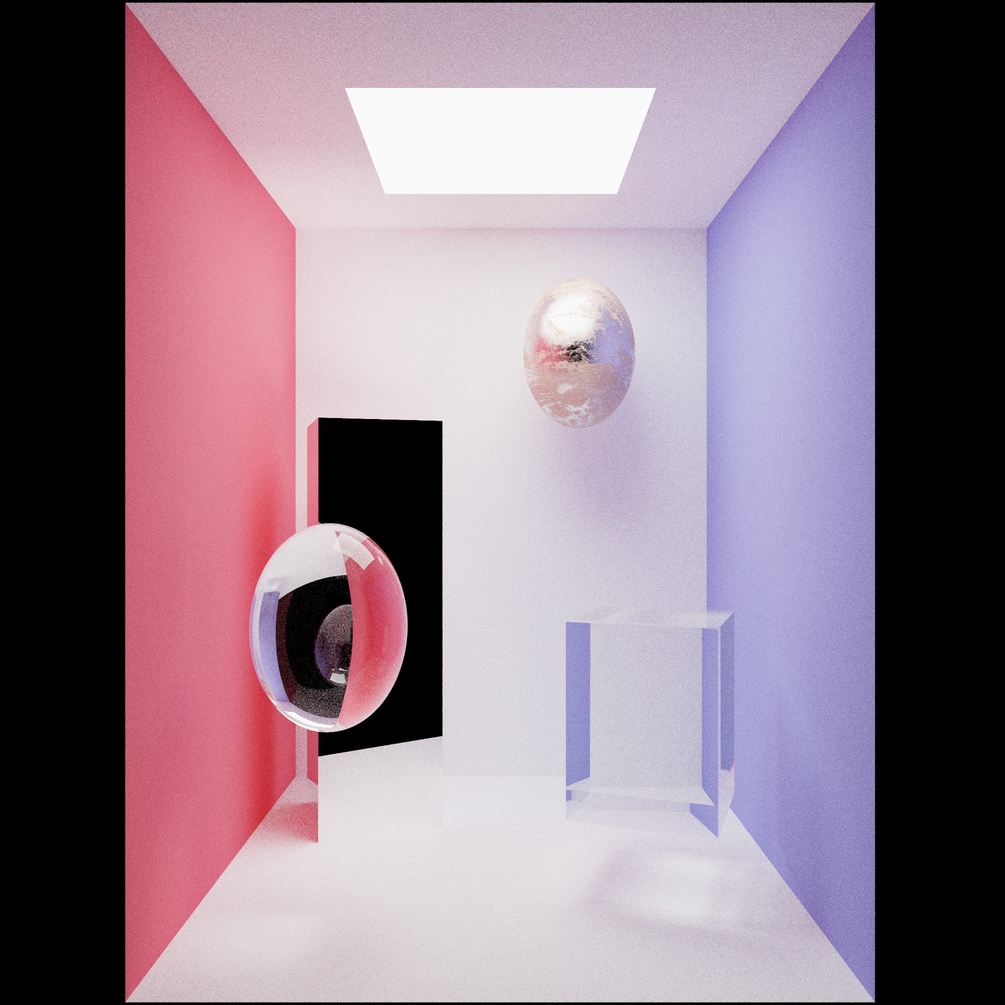
This ray tracer doesn’t use shadow surfels: at the cost of needing more samples, this method provides effects such as caustics and greatly simplifies the material system used, especially for emissive materials by not needing a separate light data structure.

A glass ball illuminated by a ball a light, left: 10 samples, right: 1000 samples.

Taking inspiration from the fantastic Physically Based Rendering: From Theory To Implementation, I’ve created a custom scene format based on JSON for loading primitives (geometry like spheres or triangle meshes) and customising their properties (like position and material).

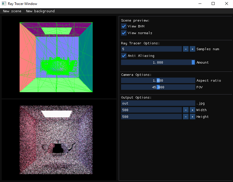
The application can be run headless to avoid some setup overhead, which is useful for creating animations, or with a GUI to debug and measure preformance.

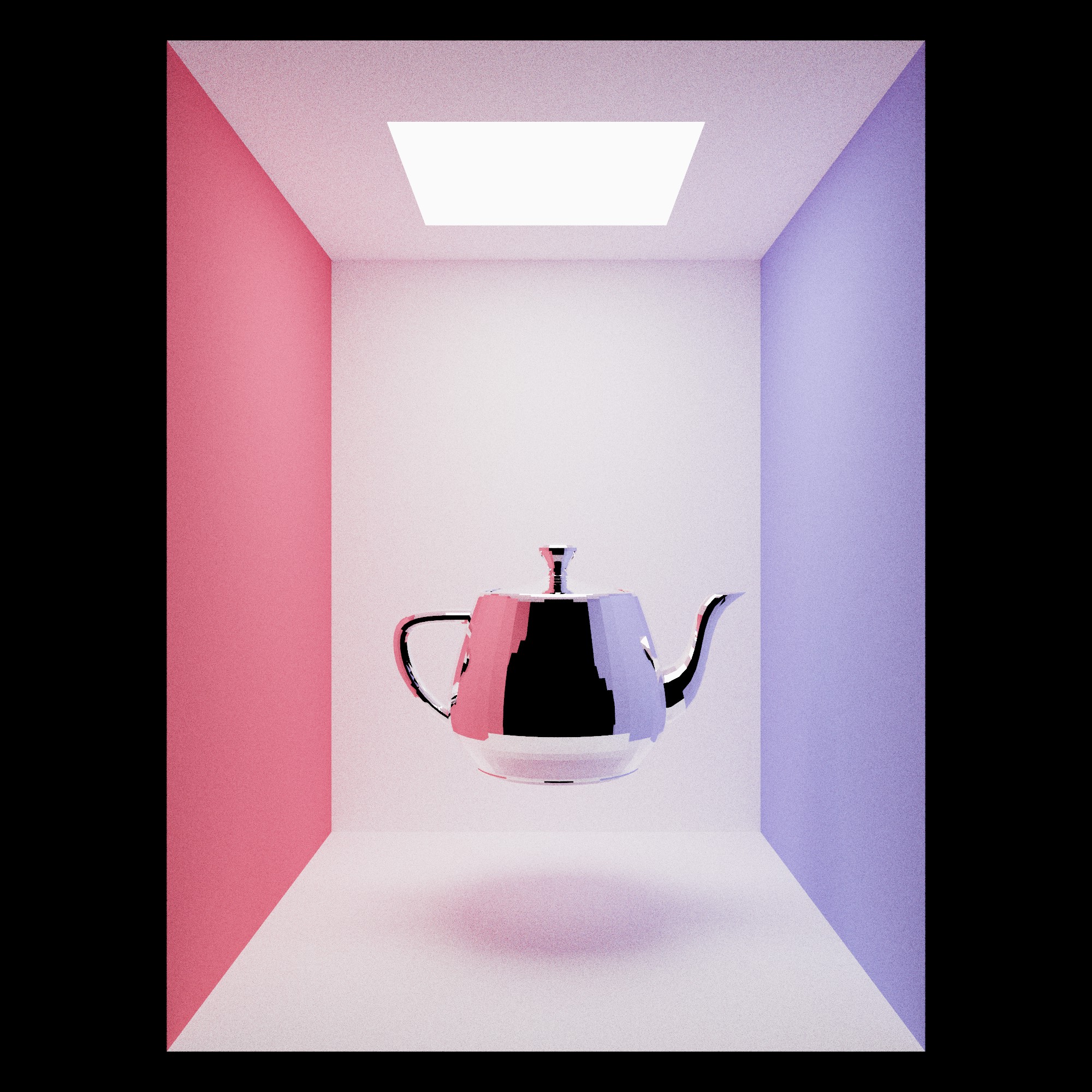Clockwise: An animation of glass balls made by a friend using my raytracer, a metal teapot in a cornell box, a rusted iron ball.

As a scene’s complexity increases, so does the need for acceleration techniques, unless one has the patience of a saint or just likes wasting their time. In this application, I have added two very common acceleration methods.

The first is an implementation of a Bounding Volume Hierarchy (BVH). I implemented a simple mid-point axis BVH, which builds a tree by recursively splitting the scene into two nodes. The split is along the axis of the mid-point of the geometric primitives within the node. I then implemented a linear BVH (LBVH), which is a bit more sophisticated but results in a faster and more reliable performance.

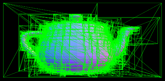From top: mid-point BVH, LBVH.

A LBVH is particulary useful for GPUs as building them is easily parallelisable. They are based on mapping “treelets”, small subtrees of scene primitives that are close together, to Morton primitives. By using these primitives, the treelets are sorted using the radix sort algorithm such that nearby treelets are in contiguous segments. We could use other sorting algorithms, but for a large number of treelets radix sort is appropriate. Furthermore, it is ideal for a GPU implementations as the algorithm doesn’t branch and works very well with SIMD.
Combined with flattening the tree into a single compact array, with nodes cache-aligned, traversal of the tree is much faster.

The second is multithreading, harnessing the multiple cores in modern CPUs and dividing the rendering task which is thankfully embarassingly parallel.

I implemented a thread pool using C++’s std::thread interface and a thread-safe, lock-based stack for processing tasks.

On initialisation, worker threads are launched with the ThreadPool::worker() function:

ThreadPool::ThreadPool(const size_t& threadCount)
    : threadCount{ threadCount ? 
    threadCount : std::thread::hardware_concurrency()},
    tasksCount{ 0 }, workers{}, running{ true }, tasks{}
{
    workers.reserve(threadCount);
    for (size_t t = 0; t < threadCount; ++t)
    {
        workers.push_back(
            std::thread(&ThreadPool::worker, this));
    }
}

void ThreadPool::worker()
{
    std::function<void()> task; 
    while (running)
    {
        // std::move from stack to task
        if (tasks.pop(task))
        {
            task();
            tasksCount--;
        }
    }
}

Thread pool initialisation and worker function.

Here are some time measurements illustrating the impact these accelerations have on the overall run-time for the same scene.

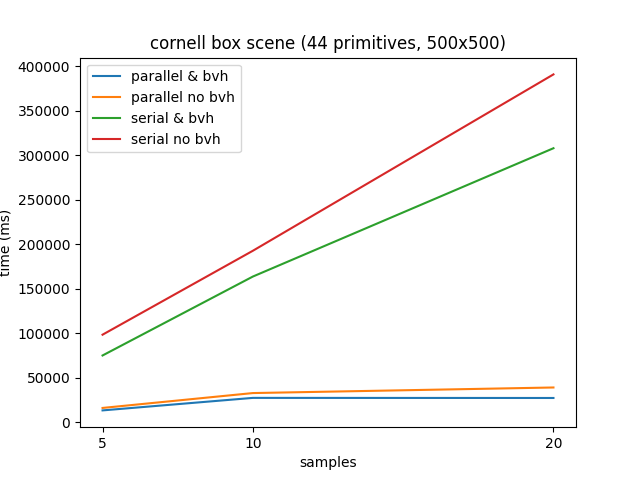Cornell box run times (averaging of 4 measurements per sample number) for the cornell box scene.

Rendering in parallel with four cores provides a consistent 600% speedup compared to serial implementations. However, because of the relatively small number of primitives in this scene the speedup provided by the LBVH, although still around 16%, is not consequential. An interesting feature of the data is the difference in standard deviation between the non-BVH and LBVH implementations which I believe is a feature of the more cache coherent BVH structure.
Whereas it seems to stabilise at around 1000 ms for the LBVH, it is much higher for the non-BVH and as large as 19775 ms for the serial implementation of 20 samples per pixel. That’s almost a 20 second difference between the slowest and fastest measurement!

Ideally for a task taking time T to complete and N cores, the application will finish in T / N.

Ray tracing an image divided equally among 4 cores.

Notice how the second image row from the bottom in the above gif finishes much later? The scene is more complex in that part of the image and the overall rendering time is bounded by the slowest thread, denying the ideal T / N runtime. This calls for a smarter division of the image amongst threads.

To help determine a better task per thread allocation, I created some heatmaps (blue = min, red = max) showing the overall complexity for a scene.

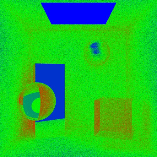
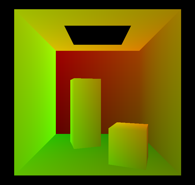
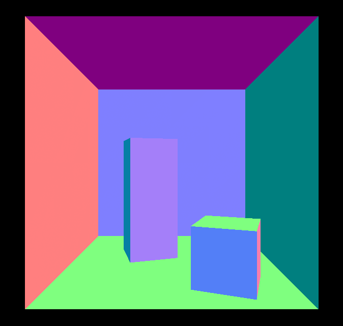
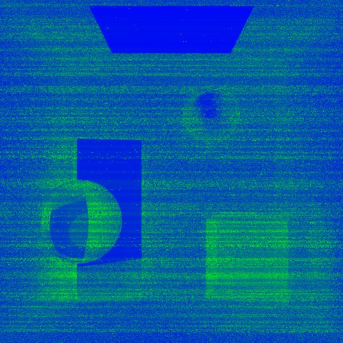Left to right (in both): heat map of ray depth, heat map of ray runtime.

This project is still very much ongoing as there is a plethora of techniques and desirable features that remain to be added!
These include:

Image Based Lighting, sample from a cube map for beautiful background reflections.
Volumetric rendering, more complex BSDFs, BTDFs and BSSRDFs.
More accurate Monte Carlo sampling for faster renders.
Vulkan GPU ray tracing.

For more information on the project and to inspect the source code, please visit the GitHub repository!